geocoder: an R package to store and access geographic data in MongoDB
L Hama
2020-02-28
Source:vignettes/geocoder-paper.Rmd
geocoder-paper.RmdIntroduction
Geocodes (Goldberg, Wilson, and Knoblock 2007) are spatial references which are used to identify points or boundaries in a geographic coordinate system. Finding geocodes is a cumbersome and repeated task for data scientists. In the case of the United Kingdom, despite the availability of “open geography portal” (National Statistics 2016), data scientists need to locate the relevant source, which could be typically an ESRI shape or sometimes a comma separated values (CSV) file. In the case of those who use R as a data science tool, this also means processing these files repeatedly. Having these geocodes handy which can be easily accessed is what geospatial database management systems (DBMS) such as PostGIS and MongoDB should be doing. The idea of having an R package that can fascilitate this is the reason for a missing R package called geocoder. In the age of availability of wide range of SQL/NoSQL and other big data oriented DBMS’es, finding geocodes should be easier.
Motivation
The Turing Institute’s eAtlas project (“Turing Geovisualization Engine” 2019) is focused on visualizing spatially referenced datasets. It would be much easier to get the geographic data from datasets using databases rather than data science workflows in R/Python. Whilst developing a web based geovisualization eAtlas and allowing users to “load” their datasets in different formats, it would be great to detect geocodes and find coordinate data (such as longitute and latitudes) “automatically”. As it stands, there is no such open API (Application Programming Interface) to query for such geographic data and availability of such data locally (to the application) is becoming a need.
Relevant technology
The standardisation of storage and access model of two-dimentional geographic references by both Open Geospatial Consortium (OGC) and International Organization for Standardisation (ISO) means programmers can define objects which represent these standards. This standard is known as Simple Features. In the case of R, the well known package called sf (Pebesma 2018) defines the standard and provides tools to manage geographic data in R. MongoDB is one of the DBMS’es which also support this standard.
MongoDB comes with built-in geospatial indexing and querying (Ameri et al. 2014) around GeoJSON (Butler et al. 2016), which is another standard built on top of Simple Featurers. MongoDB accepts GeoJSON formatted coordinates, and database indices can be created which fascilitate fast spatial queries. As a data interchange format, GeoJSON is also widely supported by mapping libraries (Page 2015). GeoJSON is JSON which is natively supported (read) by JavaScript and might be the reason for its wider popularity.
UK geocodes case
UK Office of National Statistics Open Geography Portal contains various files which are used by data scientists to plot data on maps. Details of different layers etc.
Round trip through MongoDB
To showcasee the capabilities of geocoder package, we can do a round trip data processing from a seudo-standard R spatial sf class back to itself through MongoDB’s geospatial querying. That is:
take a shapefile from UK’s Open Geography Portal and write it into a MongoDB collection and create a spatial index on it using an
sfobject.reassemble the data from MongoDB queries back to an
sfobject.
One of the UK census boundaries is called Middle Superr Output Area (MSOA), which can be found here.
msoa.folder = file.path(tempdir(), "msoa_folder")
msoa.zip = file.path(tempdir(), "msoa.zip")
if(!exists(msoa.file)) {
  download.file(
    paste0("https://opendata.arcgis.com/datasets/",
           "f341dcfd94284d58aba0a84daf2199e9_0.zip"),
    msoa.zip)
  unzip(msoa.zip, exdir = msoa.folder)
}
# read the shape file using `sf`
msoa.sf = sf::read_sf(
  list.files(msoa.folder, pattern = "England_and_Wales.shp"))
class(msoa.sf)
# substring(geojsonsf::sf_geojson(msoa.sf[1,]), 1, 350)
The data is ready in a clean sf object and we can use geocder::gc_import_sf to import into Mongodb:
We can now query the database with lists of MSOA codes and easily return GeoJSON formatted “features” ready to be reassembled into sf.
Find geocodes with spatial reference
# head(st_coordinates(st_geometry(msoa.sf[1,])))
# code for point -0.09640594 51.52283
qry <- '[
  {
    "$geoNear" : {
      "near" : { "type" : "Point", "coordinates" : [ -0.09640594, 51.52283 ] },
      "distanceField" : "dist.calculated",
      "maxDistance" : 1,
      "spherical" : true
    }
  }
] '
r = msoa.collection$aggregate(pipeline = qry)
r$properties$msoa01cd
# "E02000001" "E02000576"
The returned values are two different geometries which both correctly include the poin in the query.
Reproducible example
A reproducible (as the UK msoa example is too large) for this manuscrript would be a slice of Uber’s Vancouver land area price.
# geojson file from Uber
library(sf)
#> Linking to GEOS 3.7.1, GDAL 2.2.2, PROJ 4.9.2
v.path = file.path(tempdir(), "vancouver.json")
if(!exists(v.path)) {
  v.url = paste0("https://github.com/layik/geocoder/releases/",
                 "download/data/v10.geojson")
  download.file(v.url, v.path)
}

v = geojsonsf::geojson_sf(v.path)
vancouver = mongolite::mongo("vancouver")
# plot(v[8, ], axes = TRUE)
Let us retrieve the data and plot the land:
vancouver$drop() # if exists
geocoder::gc_import_sf(v, collection = "vancouver")
#> Writing '10' documents...
#> Registered S3 method overwritten by 'jsonify':
#>   method     from
#>   print.json jsonlite
#> There are '10' documents in collection: vancouver
#> [1] 10
r = vancouver$iterate(query = '{"properties.growth":0.2781}')
r.sf = geojsonsf::geojson_sf(r$json())
Visual check that both entries are the same:
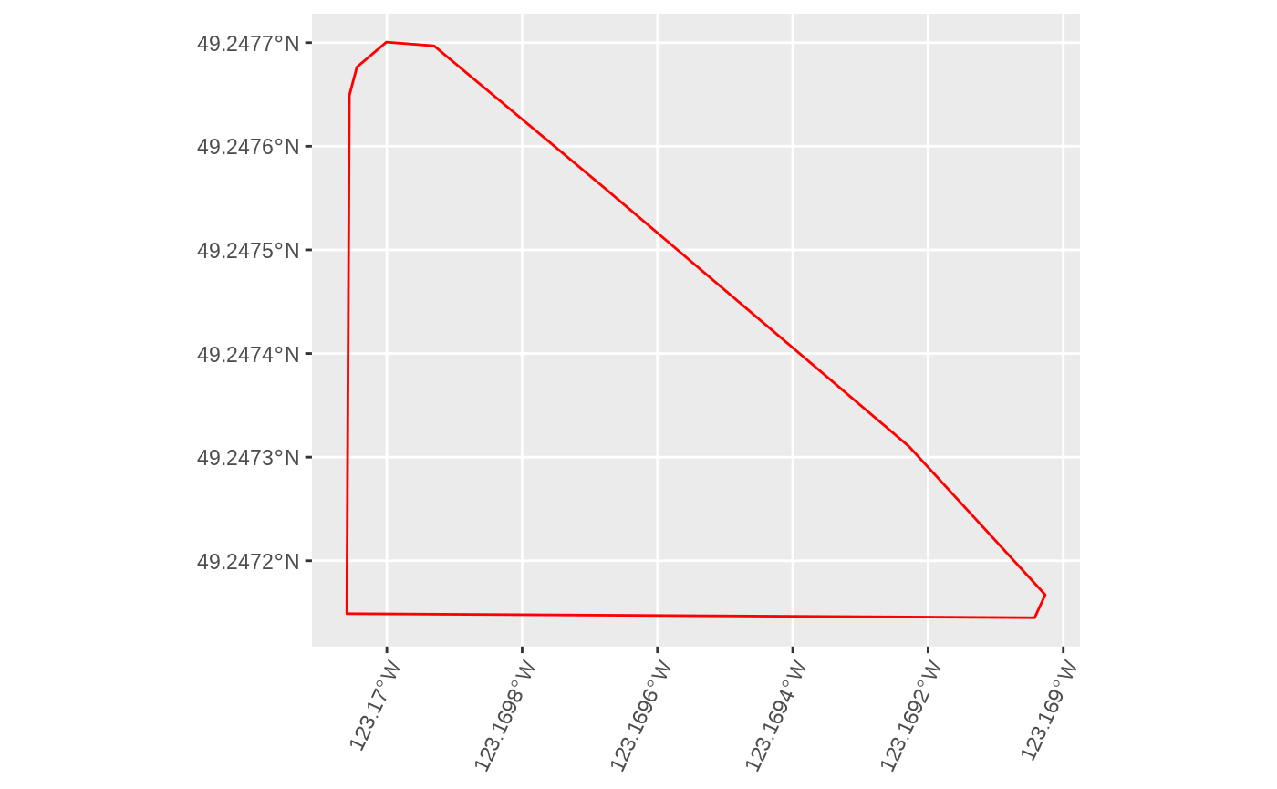

A sample from dataset plotted from MongoDB (left) and memory (right)
R vs Mongodb
We can look at a use-casee where instead of searching through geocodes in memory we query a local database. For example, instead of loadinig one ore more files and converting them into sf or similar like objecsts in R, we search an spatial index in a MongoDB instance. Lets assume you have loaded the Vancouver real estate dataset into R and the same dataset has been imported using into MongoDB using geocoder::gc_import_sf() function.
First we can make sure that a simple query returns the same number of rows:
It is also fair to assume that for a data scientist to make a spatiial query, we have to load the dataset into memory first. We know that in-memory databases are built to manage in-memory access to data, but that is not the focus at the moment.
url = paste0("https://github.com/uber-common/deck.gl-data/",
             "blob/master/examples/geojson/vancouver-blocks.json?raw=true")
v.path = file.path(tempdir(), "v.geojson")
if(!file.exists(v.path)) {
  download.file(url, destfile = v.path)
}
# sampling the data
sf = st_read(v.path)
cent = st_centroid(st_as_sfc(st_bbox(sf)))
cent = st_transform(cent, 3488)
circle = st_buffer(cent, dist = 3000)
circle = st_transform(circle, 4326)
The dataset is land boundaries in Vancouver with two variables: value per square meter and growth rate. We will use a sample of it by drawing a circle in the center of the boundary box of the whole dataset:
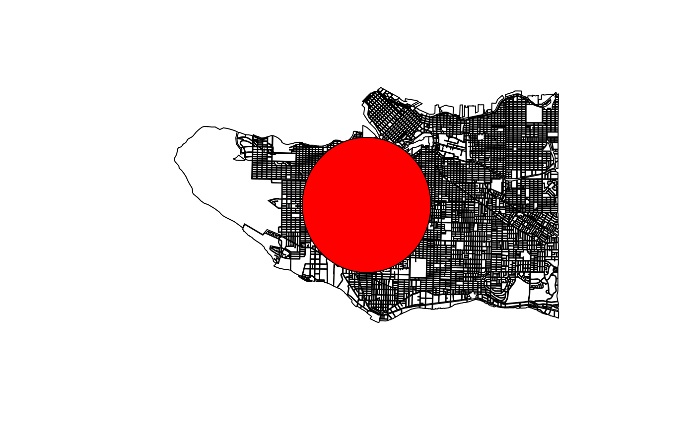
Vancouver real estate dataset and sample area.
Let us now load the dataset into MongoDB and demonstrate a basic experiment, more sophisticated and richer geospatial queries is not the focus of this document but rather to show the new R package geocoder functions:
v = mongolite::mongo(collection = "test_geocoder")
v$drop() # just in case
geocoder::gc_import_sf(sf, collection = "test_geocoder")
# scoping
sffind = NULL
vfind = NULL
# load and search
sf_search = function() {
  sf = st_read(v.path)
  # in memory search (R)
  sffind <<- st_intersection(sf, st_as_sf(circle))
}
# Mongo search
mongo_search = function() {
  vfind <<- v$iterate(paste0('{
     "geometry": {
        "$geoIntersects": {
            "$geometry": ',
             geojsonsf::sf_geojson(st_as_sf(circle), atomise = TRUE )
          ,'
        }
      }
     }'))
}
mb = microbenchmark::microbenchmark(
  sf_search(),
  mongo_search(),
  times = 1
)
Conclusion
Looking at the results, which understandably varies considerably between the two methods because in the case of searching in memory, although it is faster, we need to load the whole data (1.5mb) into memory first. To paint the whole picture, under the same circumstances, even if the whole data is queried, searching through MongoDB would only be three times slower. Figure (3) assists in doing a visual check of the two methods.
#> Unit: milliseconds
#>            expr        min         lq       mean     median         uq
#>     sf_search() 312.037108 312.037108 312.037108 312.037108 312.037108
#>  mongo_search()   1.280203   1.280203   1.280203   1.280203   1.280203
#>         max neval
#>  312.037108     1
#>    1.280203     1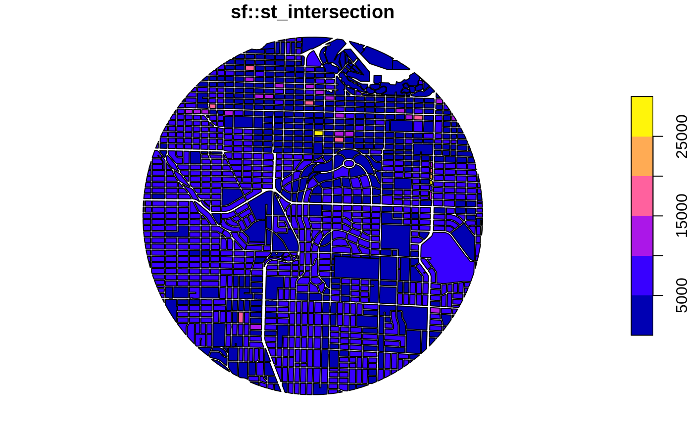
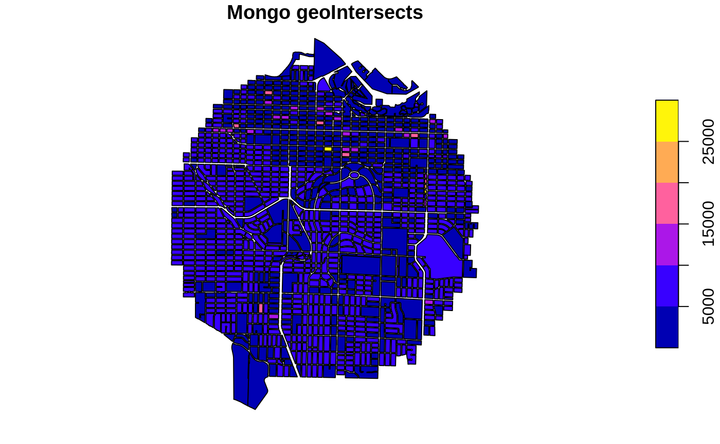
Vancouver real estate dataset sample area from sf’s intersection (left) and MongoDB geoIntersects (right). The way the two functions work can clearly be seen but the number of polygons returned are equal.
References
Ameri, Parinaz, Udo Grabowski, Jörg Meyer, and Achim Streit. 2014. “On the Application and Performance of Mongodb for Climate Satellite Data.” In 2014 Ieee 13th International Conference on Trust, Security and Privacy in Computing and Communications, 652–59. IEEE.
Butler, Howard, Martin Daly, Allan Doyle, Sean Gillies, Stefan Hagen, Tim Schaub, and others. 2016. “The Geojson Format.” Internet Engineering Task Force (IETF).
Goldberg, Daniel W, John P Wilson, and Craig A Knoblock. 2007. “From Text to Geographic Coordinates: The Current State of Geocoding.” URISA-WASHINGTON DC- 19 (1). Citeseer: 33.
National Statistics, Office for. 2016. “Open Geography Portal.”
Page, Roderic. 2015. “Visualising Geophylogenies in Web Maps Using Geojson.” PLoS Currents 7. Public Library of Science.
Pebesma, Edzer. 2018. “Simple Features for R: Standardized Support for Spatial Vector Data.” The R Journal 10 (1): 439–46.
“Turing Geovisualization Engine.” 2019. https://www.turing.ac.uk/research/research-projects/turing-geovisualization-engine.