Introducing geocoder

L Hama

2020-02-28

Introduction

geocoder R package aims at managing large amounts of geocodes easier. Instead of loading geocodes from storage formats like shape, geojson etc, it is easier for data analysts to have access to their own offline/remote database of geocodes.

UK geocodes case

UK Office of National Statistics Open Geography Portal contains various files which are used by data scientists to plot data on maps. Details of different layers etc.

Round trip through MongoDB

To showcasee the capabilities of geocoder package, we can do a round trip data processing from a seudo-standard R spatial sf class back to itself through MongoDB’s geospatial querying. That is:

• take a shapefile from UK’s Open Geography Portal

• turn it into an sf object

• write it into a MongoDB collection and create a spatial index on it.

• reassemble the output from find queries back to an sf object.

One of the UK census boundaries is called Middle Superr Output Area (MSOA), which can be found here.

msoa.folder = file.path(tempdir(), "msoa_folder")
msoa.zip = file.path(tempdir(), "msoa.zip")
if(!exists(msoa.file)) {
  download.file(
    paste0("https://opendata.arcgis.com/datasets/",
           "f341dcfd94284d58aba0a84daf2199e9_0.zip"),
    msoa.zip)
  unzip(msoa.zip, exdir = msoa.folder)
}
# read the shape file using `sf`
msoa.sf = sf::read_sf(
  list.files(msoa.folder, pattern = "England_and_Wales.shp"))
class(msoa.sf)
# substring(geojsonsf::sf_geojson(msoa.sf[1,]), 1, 350)

The data is ready in a clean sf object and we can convert each row into a ready to be used by geocder to import into Mongodb:

geocoder::gc_import_sf(msoa.sf, collection = "msoa")

We can now query the database with lists of MSOA codes and easily return GeoJSON formatted “features” ready to be reassembled into sf.

r = gc_find(data.frame(properties.msoa01cd="E02000998"), collection = "msoa")
class(r)
# [1] "data.frame"
substr(r, 1, 200)
# [1] "Feature"
# [2] "list(objectid = 998, msoa01cd = \"E02000998\", ..."

Find geocodes with spatial reference

# head(st_coordinates(st_geometry(msoa.sf[1,])))
# code for point -0.09640594 51.52283
qry <- '[
  {
    "$geoNear" : { 
      "near" : { "type" : "Point", "coordinates" : [ -0.09640594, 51.52283 ] },
      "distanceField" : "dist.calculated",
      "maxDistance" : 1,
      "spherical" : true
    }
  }
] '
r = msoa.collection$aggregate(pipeline = qry)
r$properties$msoa01cd
# "E02000001" "E02000576"

The returned values are two different geometries which both correctly include the poin in the query.

Reproducible example

A reproducible (as the UK msoa example is too large) for this Rmarkdown document would be a slice of Uber’s Vancouver land area price.

# geojson file from Uber
library(sf)
#> Linking to GEOS 3.7.1, GDAL 2.2.2, PROJ 4.9.2
v.path = file.path(tempdir(), "vancouver.json")
if(!exists(v.path)) {
  v.url = paste0("https://github.com/layik/geocoder/releases/",
                 "download/data/v10.geojson")
  download.file(v.url, v.path)
}

v = geojsonsf::geojson_sf(v.path)
vancouver = mongolite::mongo("vancouver")
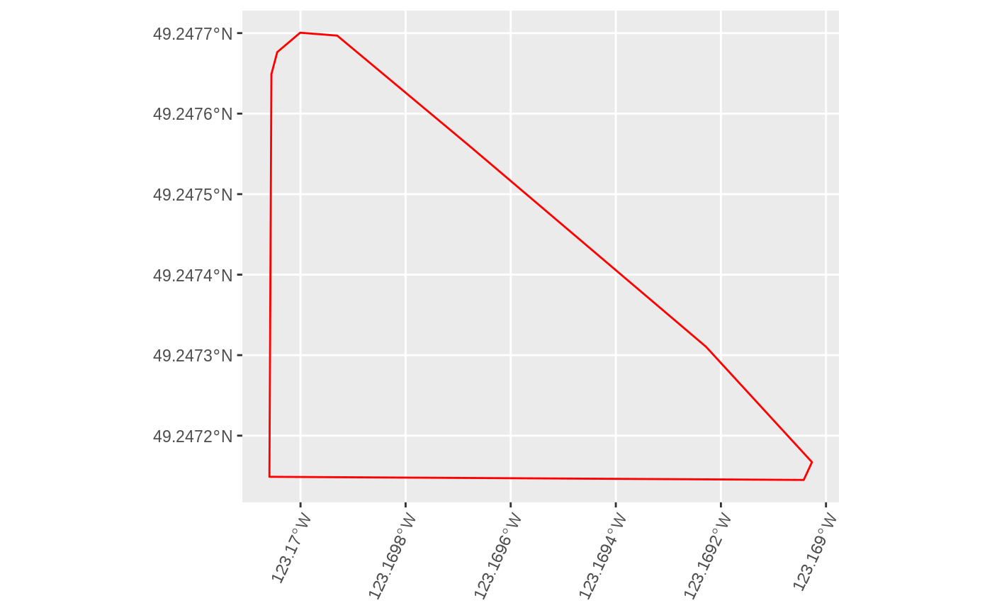
# plot(v[8, ], axes = TRUE)

Let us retrieve the data and plot the land:

vancouver$drop() # if exists
geocoder::gc_import_sf(v, collection = "vancouver")
#> Writing '10' documents...
#> Registered S3 method overwritten by 'jsonify':
#>   method     from    
#>   print.json jsonlite
#> There are '10' documents in collection: vancouver
#> [1] 10
r = vancouver$iterate(query = '{"properties.growth":0.2781}')
r.sf = geojsonsf::geojson_sf(r$json())
# plot(r.sf[, ], axes = TRUE)

Visual check that both entries are the same: